Dynamic Programming is Simple
Series:
- Dynamic Programming is Simple (this article)
- Dynamic programming is simple #2
- Dynamic programming is simple #3 (multi-root recursion)
- Dynamic programming is simple #4 (bitmap + optimal solution reconstruction)
You can use the same pattern for solving 90% of DP problems. You can find this DP pattern below.
Many people struggle with DP problems. That often happens because of the common misconception that to come up with the solution for the DP problem, you should magically discover a way to construct a table then decide a way you traverse this table, and then you magically have an answer.
Of course, if you try to think about every new problem this way, you’ll unavoidably fail and develop a strong feeling that DP is complex. Even I would run into this conclusion trying to solve the problems like this. And this is usually the approach you’re going to see in most of the solutions on LeetCode in the discussion section, which makes you feel even worse about yourself and your problem-solving skills.
However, the good news is that things are not that bad in 90% of cases. You can, and you will be able to solve 90% of DP problems without even thinking about it after some practice. The approach I’m explaining here is that it doesn’t require any insight or complex ideas. You just follow the script.
This article will give little new information if you can already solve DP problems. But if you’re still new to DP, I promise this will be extremely useful for you.
Before We Start
I’m going to ask one thing before we start. It will sound silly, but try to forget everything you knew about DP before. Like all those table-building techniques and stuff. That is not necessary at all. There are still tables, but they will come up naturally as a side effect of the solution.
We’ll be discussing the solution to this problem here: Best Time to Buy and Sell Stock with Transaction Fee
Bruteforce Solution
As with almost every algorithm problem, the first thing we do is produce a brute-force solution. You’ll later see that this is an essential part of every DP problem.
Usually, we have to come up with an idea of what we do at each step. In other words, if we end up in some state, what are our next possible moves?
For this particular problem, our options are pretty obvious. It’s either we:
- Buy stock (if we haven’t bought it yet)
- Sell stock (if we have a stock to sell)
- Do nothing (regardless if we have a stock or not)
We make the decision every day (let’s call a position in the prices array a “day” for simplicity).
So let’s say we can somehow guarantee that the state we find ourselves in is valid. Then it is quite easy to write the recurrent relation in form of recursion:
def dp(pos: int, bought: bool) -> None:
    if not bought:
        # Buy stock
        dp(pos + 1, True)

    if bought:
        # Sell stock
        dp(pos + 1, False)

    # Do nothing
    dp(pos + 1, bought)
I want to emphasize here that this is not the solution yet. This listing shows the way we branch our recursion. By doing an action every day, we move ourselves to the next state, which is itself valid.
There is nothing wrong with buying or selling stocks if we can do so. So the important thing to recognize here is that every branch of our recursive calls brings us to a new valid state, from where we can branch further.
Now we’re halfway to the final solution. It does not look like that, does it? You used to think about DP in terms of some tables and stuff. And now the only thing you see is some recursion which kind of makes sense, but how could it be a DP solution? Patience, it will become apparent in the next couple of minutes.
At this point, the function does not return anything yet. We need to fix it. And add a base case, of course. Otherwise, our recursion will run indefinitely.
The problem description asks us to find the maximum profit. So what if we say that the return value of every recursive call is itself a maximum profit starting from this “day”? How do we keep the contract and return the correct value now?
To calculate the correct value to return, we should get back to the problem description and think about how certain operations change our profit. So:
- When we buy a stock, we spend money (pay the fee) and therefore decrease whatever profit we get from the next recursive call.
- When we sell the stock, we get money back, thereby increasing profit.
- When we do nothing, profit does not change.
Applying these operations to maximum profits returned from subsequent recursive calls, we get all possible profits we can get from here.
Now we just want to get the maximum profit from all 3. That will be our new maximum profit, which is valid since the operations we have applied are perfectly valid, and we have a contract from all subsequent recursive calls we issued.
Finally, the base case: if we ran over the last day, the maximum profit we can get is 0 for obvious reasons. So the base case is valid.
And now we have full proof by mathematical induction that our algorithm is correct.
With that, let’s finish our code for the brute-force solution:
class Solution:
    def maxProfit(self, prices: List[int], fee: int) -> int:
        def dp(pos: int, bought: bool) -> int:
            if pos >= len(prices):
                return 0

            profit = 0

            if not bought:
                # Buy stock
                profit = max(profit, dp(pos + 1, True) - prices[pos] - fee)

            if bought:
                # Sell stock
                profit = max(profit, dp(pos + 1, False) + prices[pos])

            # Do nothing
            profit = max(profit, dp(pos + 1, bought))

            return profit

        return dp(0, False)
As we proved earlier, this is a perfectly valid solution, and it gives the correct result. It is not optimal, though, and therefore not a DP solution yet (I’ll leave it to the reader to estimate the complexity of this solution). But we’re one line away from the DP solution. So let’s move forward.
Top-Down DP Solution
Now we have to notice that the function dp has only two arguments: pos and bought.
Let’s try to draw a tree of all the calls we make for the following input.
prices = [1,3,2,8,4,9], fee = 2
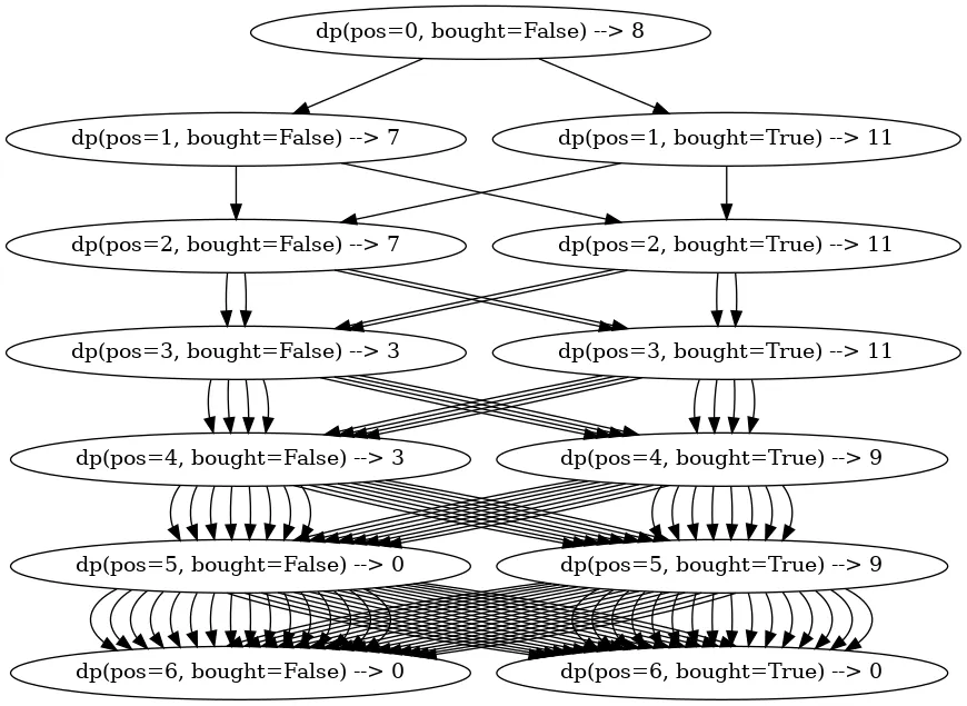
As is clearly visible from this picture, we run into the same calls all the time. That happens because pos can take up to N values (size of the prices array), and bought can take two values (True or False). So there are 2 * N possible inputs for the dp(pos, bought) functions. That means that when we fan out down the recursion, we’ll run into some of the inputs multiple times.
The function with the same input should return the same result as it does not depend on anything else. So what we can do here is to cache the return value for the function call.
In Python, it is super easy. We just have to add the lru_cache decorator on top of our function:
from functools import lru_cache

class Solution:
    def maxProfit(self, prices: List[int], fee: int) -> int:
        @lru_cache(None)
        def dp(pos: int, bought: bool) -> int:
            if pos >= len(prices):
                return 0

            profit = 0

            if not bought:
                # Buy stock
                profit = max(profit, dp(pos + 1, True) - prices[pos] - fee)

            if bought:
                # Sell stock
                profit = max(profit, dp(pos + 1, False) + prices[pos])

            # Do nothing
            profit = max(profit, dp(pos + 1, bought))

            return profit

        return dp(0, False)
And this is already a DP solution. We call this a Top-Down solution because we start from the top of the recursion tree and go down step by step.
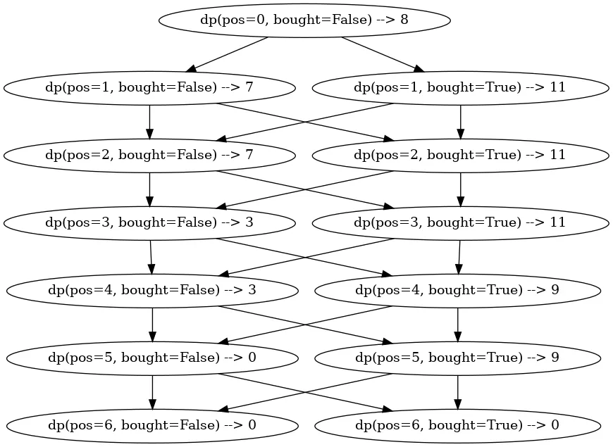
The call graph for this solution looks much better! And the complexity of this solution is O(N) because we now make a call with each combination of function arguments only once.
So, as you see, there is no magic here at all. DP is just a matter of writing what is stated in the problem description in the form of a recurrent relation (recursion) and caching the output.
It will come to you with practice, what exactly you have to select as arguments to the function and how to build a recursion.
But anyway, the main idea here is that DP is no magic at all. We have not built any tables yet (as many people do) and did not try to come up with some complicated way to go over this table. We simply have written down what’s obvious.
Bottom-Up Solution
Even though we already have a valid DP solution, there are ways to make this solution even better.
That is where those tables you heard about before are coming into play. The lru_cache we have used for caching the solution can be represented as a table.
We can initialize a cache table like this (position pos goes on the horizontal axis, bought on the vertical)
      0  1  2  3  4  5  6
true  0  0  0  0  0  0  0
false 0  0  0  0  0  0  0
Then we can use this table to cache the values we get from dp() function calls.
And then, we can go even further and make the code non-recursive.
For that, let’s look at what types of recursive calls we make:
(pos, bought) -> (pos + 1, True)   # if bought == False
(pos, bought) -> (pos + 1, False)  # if bought == True
(pos, bought) -> (pos + 1, bought)
This means if we want to calculate the value for pos, we need first to calculate values for pos + 1.
Using this information, you can already easily write an iterative solution yourself. As an exercise, you can try to do it or continue if you’re impatient.
Now I’ll give you a small trick to write the iterative solution without any effort at all. If you have a recursive solution already (and we do), all you have to do is:
- Create a
dptable having the size to fit all the cached values ofdp()function calls - Replace
dp()function definition by a loop over all possible values of arguments. Here you have to be careful with the looping order. You have to go back over theposargument because you need to calculatepos + 1before calculatingpos. - Replace
dp()function calls with calls to thedptable we have created before. - Replace
returncall by settingdpcache value. - Remove a base case as it is not needed anymore, and make sure you’ve initialized the
dptable with values that cover the base case.
Applying all the transformations above, we get the following code:
class Solution:
    def maxProfit(self, prices: List[int], fee: int) -> int:
        dp = [[0] * (len(prices) + 1) for _ in range(2)]

        for pos in range(len(prices) - 1, -1, -1):
            for bought in range(2):
                profit = 0

                if not bought:
                    # Buy stock
                    profit = max(profit, dp[1][pos + 1] - prices[pos] - fee)

                if bought:
                    # Sell stock
                    profit = max(profit, dp[0][pos + 1] + prices[pos])

                # Do nothing
                profit = max(profit, dp[bought][pos + 1])

                dp[bought][pos] = profit

        return dp[0][0]
This code is a correct Bottom-Up DP solution. We call it this way because instead of going from the root of the recursion tree, we calculate leaf values instead and then go up layer by layer.
The time complexity of this solution is O(N), and memory complexity is O(N) as well.
At this point, we can stop as it is already a correct iterative solution. But we can do even better.
Bottom-Up Solution (Optimized)
To further optimize the solution, we notice that if we want to calculate the values for pos, we need to calculate only values for pos + 1 and nothing else. Like we don’t need values at pos + 2 etc. So we can throw away everything else.
That leads to another solution:
class Solution:
    def maxProfit(self, prices: List[int], fee: int) -> int:
        dp = [0] * 2

        for pos in range(len(prices) - 1, -1, -1):
            new_dp = [0] * 2

            for bought in range(2):
                profit = 0

                if not bought:
                    # Buy stock
                    profit = max(profit, dp[1] - prices[pos] - fee)

                if bought:
                    # Sell stock
                    profit = max(profit, dp[0] + prices[pos])

                # Do nothing
                profit = max(profit, dp[bought])

                new_dp[bought] = profit

            dp = new_dp

        return dp[0]
That is the perfect solution the interviewer is looking for.
The time complexity is still O(N), while the space complexity is O(1).
Final Thoughts
As you hopefully see now, DP is very straightforward. There are no complex ideas required to solve such problems. You just have to build a brain muscle that will allow you to build the initial recurrent relation correctly. The rest is about caching the recursive calls and turning the solution upside down so we get an iterative solution.
Let’s reiterate the steps we have done to build the solution:
- Decide what we have to do at each step to bring us to the next valid state. Write down the recursive calls that implement this behavior.
- Come up with a way to construct the next optimal solution with all the data you got from subsequent recursive calls. Add a base case and complete the recursive function. Now you have a brute-force solution.
- Notice you have a limited set of possible arguments combinations and cache the return values, so you avoid calling the function twice with the same arguments. This is a Top-Down solution.
- Using the rules described in the article, convert the Top-Down solution to the Bottom-Up solution.
- Look closer at what data you use on each step. Maybe you don’t need it all, and you can optimize your code memory-wise. This is not always the case, though. Sometimes it is impossible.
From my experience, it takes about 15-20 DP problems to master this method. It might look hard initially, but later you will see that all DP problems are the same, no matter if they are medium or hard level on LeetCode. Also, you will start recognizing DP just by reading the description. If the description of the problem has:
- Directions on what to do on each step (buy/sell a stock, insert/delete/replace/keep character, etc.)
- The requirement to find minimum/maximum
You will know for sure it is a DP problem, and in the next 30 seconds, you will build a solution in your head.
Of course, there are exceptions, but in general, 90% of DP problems look exactly like this one. If there are requests, I can describe those exceptions and slight divergences from this pattern in the next article.
So don’t be afraid of DP problems. Everybody can master those problems. And they are much more manageable than most of the problems of a similar level.
I wish the best of luck to everybody who has read till here. I hope this was helpful for you.
PS: You can find all the solutions from this article here. And there are solutions for much more problems if you check the readme doc of the repo.
This article is also available on Medium.